A 905 nm micro-pulse photon-counting LiDAR that reads Mars's dust and
cloud profiles from the ground — designed end to end, from a closed link budget down to the
40 A gallium-nitride pulse loop, and standing in the city as a live asset that fires a
visible probe beam. Beside it stands an optical observatory whose 512×512 photon-counting
focal plane exists only because seven rounds of device physics turned a dark-count problem
into a sub-hertz one.
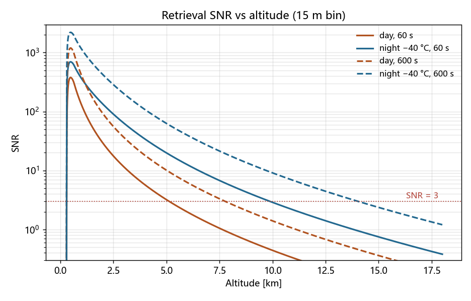
Night range
14.0km · 600 s
Daytime range
5.1km · 60 s
Focal plane
512²SPAD · 15 µm
Dark count, all-T
0.383Hz/px
01
What it is
A single-site atmospheric LiDAR: point a low-energy pulsed laser straight up,
count the photons that scatter back off dust and ice, and invert the echo into a vertical
profile.
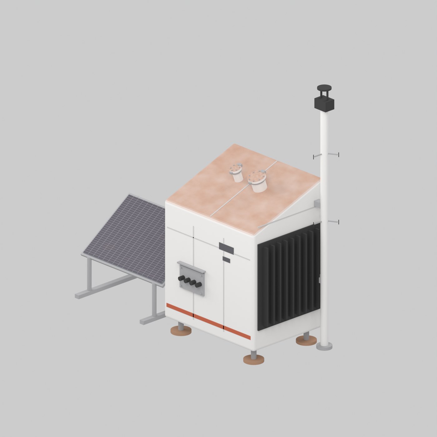
The station is a wedge enclosure barely 1.6 m across, tilted-roof to shed dust, with
two optical ports on top — a transmit beam expander and a Ø125 mm receive telescope —
a nine-fin radiator wall, four leveling feet, a tilted solar panel, and a 3.5 m weather
mast. Everything electrical lives inside: three custom boards, an FPGA, a battery.
It runs a micro-pulse, photon-counting regime: 3 µJ pulses at
9.5 kHz rather than one big shot, so the average launched power is only
28.5 mW. Sensitivity is bought back with high repetition and long
integration — which is exactly what lets the whole station run off a small solar panel.
In the city it is asset sci-lidar-01, built as real-metric
three.js geometry that emits a 905 nm probe beam off its 20° roof.
SCI-LIDAR-01 — 1.6 m WEDGE ENCLOSURE · TWIN ROOF PORTS · 3.5 m WEATHER MAST
And next doorThe optical observatory
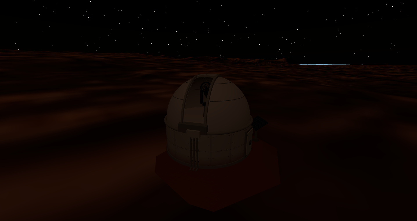
A 6 m hemispherical dome on a compacted-regolith plinth, with a dust-sealed
up-and-over slit shutter. Inside, a 200 mm f/5 Ritchey–Chrétien on an
alt-azimuth fork looks out through the slit. At dusk the shutter leaf rides along its rails
over the zenith and parks on the back of the dome; the dome then slews slowly through the
night and reseals at dawn. That is real articulation in the city model, not a painted
texture — shutter, dome azimuth and telescope elevation are named joints the engine drives.
A 20 cm aperture sounds modest until you account for where it stands. The Martian
atmosphere is 0.6 % the density of Earth's, so seeing is close to
space-like: the 0.7″ diffraction limit sits well inside a 3.09″ pixel, and the pixel — not
the air — sets the resolution. What makes the instrument interesting is not the mirror. It is
that everything downstream of the first photon was designed here: the detector, the readout
chip, its layout, the optics and the thermal path.
SCI-OBS-01 AT NIGHT — SHUTTER OPEN, OTA VISIBLE THROUGH THE 1.25 m SLIT
02
How it works
A biaxial transmit/receive pair, and the two things that decide where it can
actually see: the geometric overlap near the ground, and the noise floor far away.
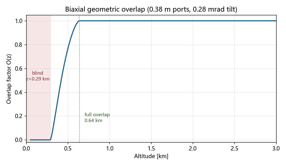
Transmit and receive sit side by side, port centers 0.38 m apart, the
laser tilted 0.28 mrad inward so the narrow beam walks into the
receiver's field of view. That geometry gives a hard blind zone below
0.29 km and full overlap by 0.64 km — pulling
the ports closer than the first design (0.76 m) is what lowered the blind floor.
Far away, the limit is background: a 0.3 nm filter and a 1 mrad field stop knock
down the daytime sky so a single returning photon still clears threshold. The detector is a
cooled silicon SPAD array (the device end, below); the receiver front end turns one
photoelectron into a 16 mV pulse and discriminates it at a half-photoelectron
threshold. The FPGA histograms arrivals into 1000 range bins of 15 m each — a
15 km window.
RETRIEVAL SNR — NIGHT −40 °C REACHES 14.0 km @ 600 sBIAXIAL OVERLAP — BLIND BELOW 0.29 km, FULL BY 0.64 km
03
The detector
At the heart of the receiver is a purpose-built near-infrared SPAD array —
its own device-physics story.
The array is nir_iproc_p10j, a 1×1 mm silicon photon counter
(625 cells) developed on the spad40 process line and frozen for this instrument. Its 905 nm
photon-detection efficiency, dark-count floor, and breakdown behavior were closed out in TCAD
and feed directly into the link budget above.
Section owned by the spad40_nir device session
Device-physics figures and the TCAD ledger (PDE(V), dark-count trimming,
McIntyre breakdown, Geiger transient) are supplemented here by the spad40_nir session. The
system-level delivered values it hands off — PDE@905 40.3%, back-to-back floor
253 cps·cell⁻¹, array DCR 2.65×10⁵ cps @ −40 °C — are the inputs the numbers
above are built on.
04
The observatory, from the photon inward
Four design problems in series. Each one changed the answer to the next.
04 · AThe detector had to be invented first
Photon-starved astronomy is a dark-count problem before it is anything else. The budget was
under 1 Hz per pixel. The first real-process port of the parent SPAD sat at
a peak multiplication field of 6×10⁵ V/cm — deep in band-to-band tunnelling
territory. A dose sweep measured the law: dark count ×10 for every
0.29×10⁵ V/cm of peak field. Reaching 1 Hz in a 15 µm pixel
needs ≤4.24×10⁵ V/cm — but at that field the sharp junction's trigger
probability collapses below 0.5. Trimming the implant dose cannot close this budget.
That negative result is what forced an architectural change.
The fix is to buy the ionization integral with width instead of field:
insert a low-doped gap between the charge sheet and the substrate so the gap carries a flat
field E = qN/ε. Two knobs then control everything — retained dose
sets the field, buffer thickness sets the multiplication width. Seven process rounds and
about eighteen device variants later, iwK115 lands at
4.33×10⁵ V/cm across a 0.74 µm multiplication width, trigger probability
0.904, and a measured band-to-band floor of
0.383 Hz per 15 µm pixel.
Two consequences fell out of that geometry. Because the operating field is set by the
retained charge rather than by the bias, it is temperature-independent — so a
single fixed 88 V serves the whole 120 K diurnal swing and the bias-tracking servo a
classical SPAD needs is simply deleted. And because a wide-multiplication device has a large
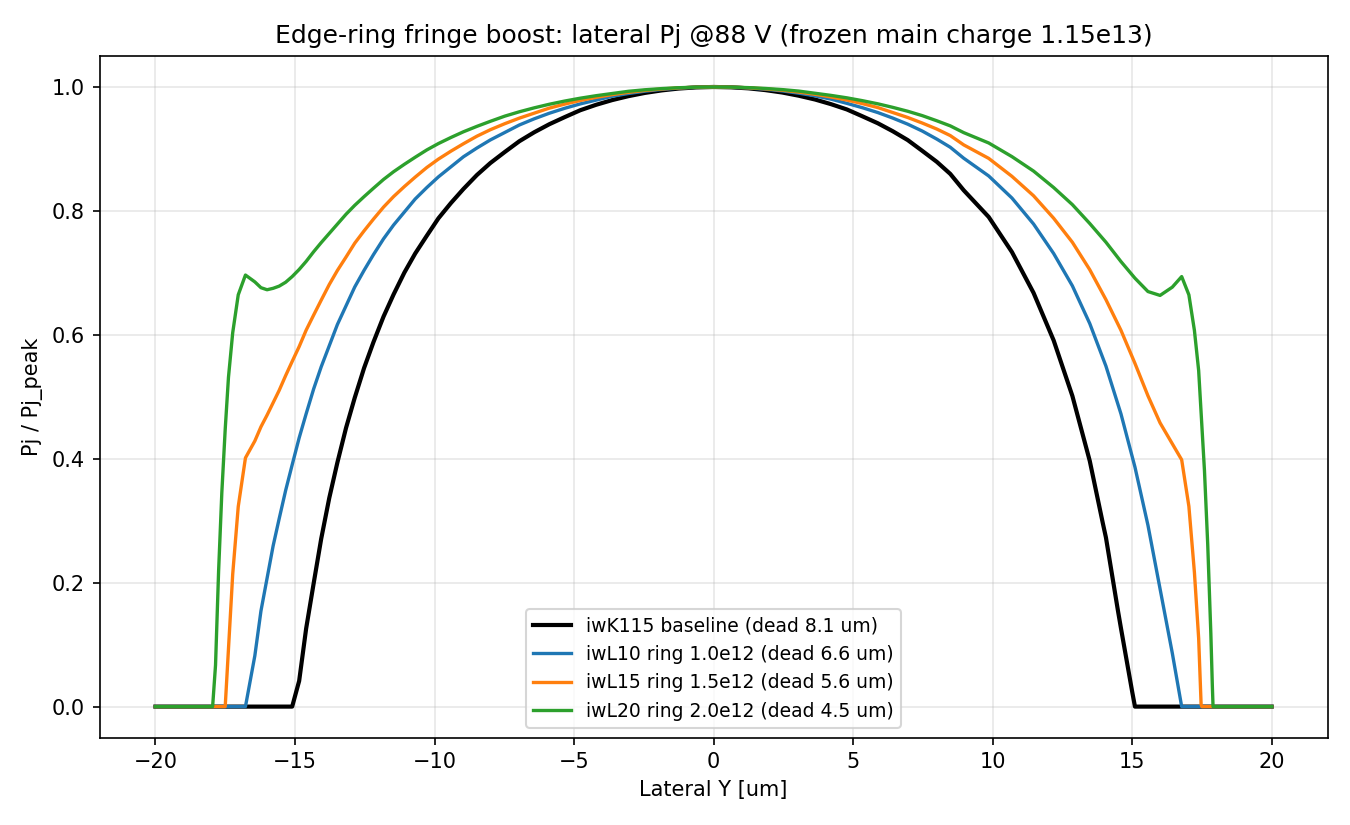
lateral roll-off, an 8.14 µm dead border per side would have eaten a 15 µm pixel
alive: a light 2.0×10¹² edge-ring implant shrinks it to 4.45 µm/side for
+1.3 % centre field. A microlens then decouples fill factor from pitch entirely — 15 µm
with a microlens (0.88 effective) beats a bare 40 µm pixel (0.79) while cutting dark
volume and radiation-damage rate about sevenfold.
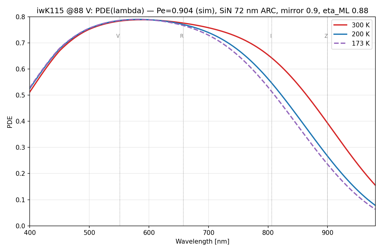
IWK115 PDE(λ) AT 173 K — V 0.79 / R 0.77 / I 0.51 / Z 0.24EDGE RING — DEAD BORDER 8.14 → 4.45 µm/SIDE AT +1.3 % CENTRE FIELD
04 · BA readout chip that never sees high voltage
The partition came before the circuit. The quench divider — 3.6 MΩ and 270 kΩ of
hi-res poly — stays on the SPAD die, so 88 V and the full avalanche swing never leave it.
The readout ASIC's highest rail is 3.3 V, and exactly one high-voltage
line exists in the whole instrument. Several mechanical and safety margins later on this page
are downstream of that single decision.
Each pixel is a two-stage 3.3 V sense inverter, a level shifter and a toggle
flip-flop — one bit of frame memory, read at 1 kHz. Photon rate is
recovered off-pixel from the parity statistics,
λ = −ln(1−2p̄)/(2T_f), which costs 0.26 Gbps for a 512² array
and needs no counter, no ADC and no analog column chain. A bright star saturates parity at
p→0.5 and reads as a flat top instead of wrapping around, and the flip-flop doubles as the
scan latch.
The silicon is drawn by Python generators that emit Cadence SKILL, then verified with
Calibre: 12 cells, DRC 0 on every one, LVS CORRECT 11 of 11. The pixel is
12.0 × 16.0 µm drawn on a 14.97 µm rail pitch, mirror-tiled so neighbouring rows
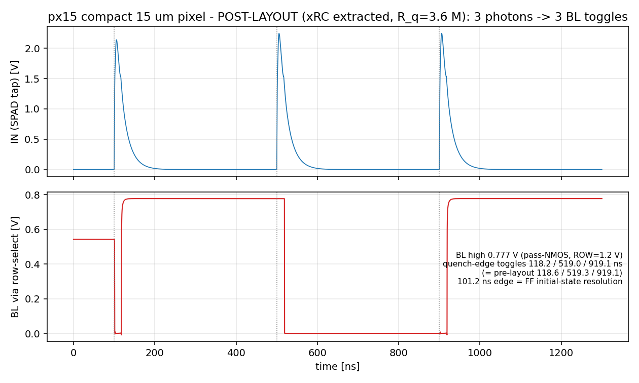
share power rails. After parasitic extraction, three photons produce three bit-line toggles
at 118.2 / 519.0 / 919.1 ns against a pre-layout 118.6 / 519.3 / 919.1 —
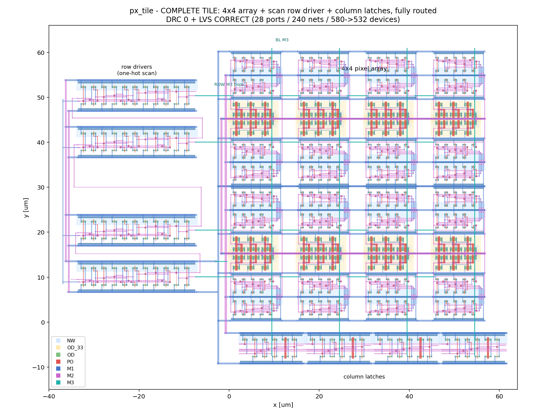
agreement within 0.5 ns through the real RC. The complete tile
(4×4 array + one-hot scan row driver + column latches, fully routed) closes at 28 ports,
240 nets and 580→532 devices.
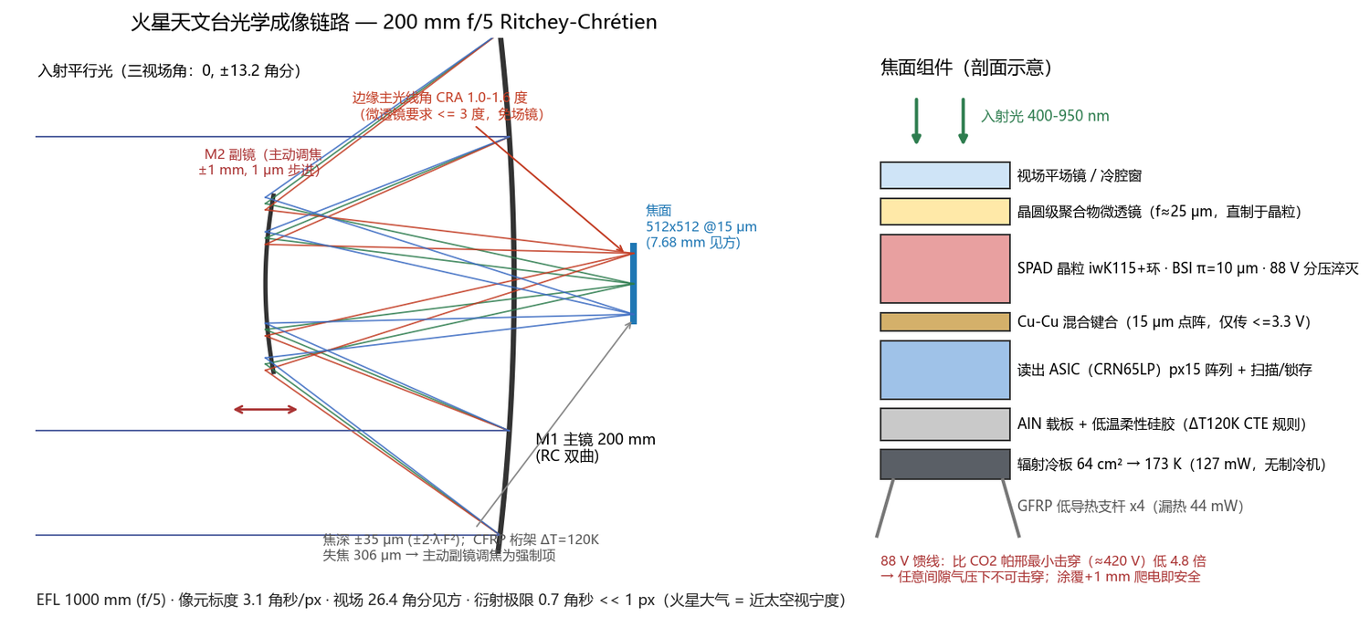
The telescope is sized to the sensor rather than the other way round: 200 mm f/5,
1000 mm focal length, giving 3.09″ per pixel over a 26.4′ square field.
The microlenses impose a chief-ray-angle limit of 3°, and plain geometry meets it — an exit
pupil 200–300 mm from the focal plane puts the edge chief ray at 1.0–1.6°, so no field
lens is needed.
Focus is the unforgiving one. Depth of focus is ±35 µm, while a CFRP metering truss
drifts 306 µm over the 120 K day–night swing once secondary magnification
multiplies it seventeen times. Invar overshoots by 26×, aluminium by 402×. No passive
structure survives, so an active secondary focuser is mandatory — ±1 mm
travel, 1 µm steps, driven from a temperature table and trimmed on a star at the start
of each night.
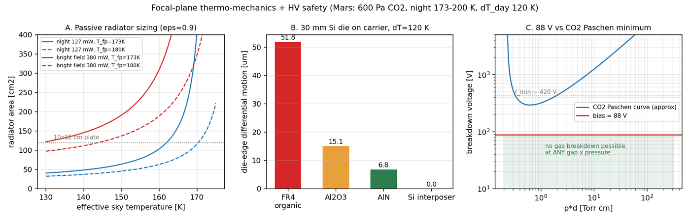
Cooling, by contrast, is nearly free. The whole cold assembly dissipates
127 mW at night — and only 2.5 mW of that is the detector array;
struts and harness account for 94 mW. A 64 cm² passive radiator holds the focal
plane at 173 K with no cryocooler and no heater loop, because the fixed-bias device
tolerates the whole temperature range anyway.
Three integration rules fell out of those budgets. The die carrier must be AlN or a
silicon interposer — an organic carrier shears 51.8 µm at the edge of a 30 mm die
over 120 K — and the die attach must stay compliant at 140 K (silicone 0.07 MPa;
rigid epoxy 68 MPa). The microlenses must be wafer-level replicated on the SPAD die
itself: a separate fused-silica plate spends 45 % of the ±2.1 µm alignment budget on
thermal drift alone. And the high voltage turns out to be a non-issue — 88 V sits
4.8× below the CO₂ Paschen minimum (≈420 V), so gas breakdown is impossible at any
gap × pressure combination. That is what the divider-on-the-SPAD-die partition bought.
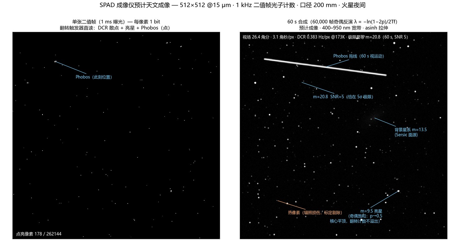
With every constant fixed by the verified design — effective aperture, 0.55 broadband PDE,
0.88 microlens fill factor, the measured 0.383 Hz/px dark rate and 1 ms binary
frames — the instrument can be simulated forward. A single frame is startling:
178 lit pixels out of 262 144, a scatter of one-bit dots in which Phobos is a
single point. Stack 60 000 of them, invert the parity, and a real sky appears: point sources
down to magnitude 20.8 at SNR 5, a Sérsic galaxy, radiation hot pixels
that calibrate out, Phobos drawn into a streak by its own motion, and the bright star sitting
there with a flat parity-saturated core instead of a bloomed, overflowed one.
SIMULATED 1 ms FRAME vs 60 s STACK — LIMITING MAGNITUDE 20.8 (SNR 5)
Optics, thermo-mechanics and imaging (analytic + forward simulation)
Plate scale / field of view
3.09″/px · 26.4′
mars_spad_rox/scripts/calc_mech_design.py
Edge chief-ray angle (pupil 200–300 mm)
1.0–1.6°
mars_spad_rox/scripts/calc_mech_design.py
Depth of focus vs CFRP thermal drift
±35 µm vs 306 µm
mars_spad_rox/scripts/calc_mech_design.py
Night heat load → radiator area
127 mW → 64 cm²
mars_spad_rox/scripts/calc_mech_design.py
Die-edge CTE shear, organic vs AlN
51.8 vs 6.8 µm
mars_spad_rox/scripts/calc_mech_design.py
Paschen margin on the 88 V feed
4.8× below minimum
mars_spad_rox/scripts/calc_mech_design.py
Limiting magnitude, 60 s stack
20.8 at SNR 5
mars_spad_rox/scripts/sim_expected_image.py
Lit pixels in one 1 ms frame
178 / 262 144
mars_spad_rox/scripts/sim_expected_image.py
Frame data rate, 512² at 1 kHz
0.26 Gbps
mars_spad_rox/docs/sensor_floorplan.md
06
What broke
The honest list — stale numbers, a short hiding as a hint, phantom opens, and
six failed process rounds.
The stale baseline. The link budget's overlap model carried a
0.76 m port separation, but the mechanical build had already pulled the two ports to
0.38 m to shrink the blind zone — and the budget never followed. A mechanical
dissection caught the mismatch; reconciling to 0.38 m nearly halved the measurable
near-field floor, from ~0.7 to ~0.4 km.
A blind zone that looked like a ceiling. Once the overlap function was
physical, the near field became a true blind zone. The range solver still took "the first
altitude where SNR < 3" and dutifully reported the blind zone as the range
ceiling — 0.6 km. Rewritten to take the highest altitude with SNR ≥ 3.
Two nets in one hole. A duplicate connector slipped through the
schematic-to-board sync, and reflowed pin-rows overlapped until a 64 V rail and ground
shared a single plated hole — a dead short that the checker only surfaced as "airwires."
Found by scanning every pad pair for coincident coordinates; fixed by de-duplicating and
spreading the connectors.
Phantom open circuits. After a batch copper push the EDA under-registered
nets and threw dozens of "No Connection" errors on traces that were physically joined.
Cleared by re-touching every trace's net assignment — then a real via-clearance handful
fell out and got fixed.
Insulation, not tuning. The 1.5 A thermoelectric driver pumps only
0.82 W across a 40 K lift, so the parasitic heat leak has to sit far below that.
The −40 °C hold is won by insulation, not by control-loop gains — a constraint the
design script surfaced before any hardware existed.
ObservatorySeven process rounds means six of them failed
The dose trim that couldn't. The obvious way to lower a dark count is to
lower the implant dose until the field comes down. Four doses were swept, the law came out
clean, and the conclusion was fatal: at the field the budget demands, the sharp junction's
trigger probability is below 0.5. The device would have been quiet and blind. Only then did
the architecture change.
Charge stacking that sharpened the field. The first attempt to widen the
multiplication region stacked three implant energies. It did the opposite of the intent —
the deep energies piled charge at the substrate junction and pushed the peak field
to 6.5–8.7×10⁵ V/cm. Width has to come from a low-doped gap, not from more
implants, and that only shows up when you plot the field rather than the doping.
The implant that evaporated. The next round moved the charge higher above
the substrate and lost 97 % of the dose through the thermal drive: the heavily doped
substrate interface acts as an interstitial sink, so charge more than ~1.3 µm away is
smeared into nothing. A later attempt to sidestep implants with an in-situ doped epi layer
was silently wiped by the next same-material deposit — the profile simply wasn't
there in the final structure, and nothing in the log said so.
Trigger probability 0.99, drift field 21 V/cm. One over-dosed variant
looked like the best device in the family until the drift field in the absorption region was
checked: it had never punched through. Voltage was piling up at the junction while the
absorber stayed undepleted, so photons were landing where nothing collected them. Trigger
probability alone is a liar; reach-through has to be verified separately.
The keeper that won. The column sense latch was drawn, DRC-clean and
LVS-clean — and could not be written. Its cross-coupled keeper was the same strength as the
transmission-gate write path, so the latch simply held its old value. A textbook
ratioed-latch error, caught the first time the cell was simulated rather than the first time
it was drawn, which is the whole argument for simulating cells.
Sixteen identical latches. A nominal transient of the fully extracted array
refused to resolve: sixteen identical flip-flops park at the same metastable point, the state
lives in nodes the extractor renamed, and the model deck carries no device mismatch to break
the symmetry. Real silicon resolves this with mismatch and a per-frame reset. Rather than
dress up a simulation that could not answer, the claim was decomposed — pixel function proven
on one cell, array connectivity proven by LVS and extraction, and the shared-column readout
proven by a deterministic preset-and-read experiment.
The 21.5 that was 20.8. Writing this page caught one of its own numbers.
The imaging figure had carried a limiting magnitude of 21.5 in its caption since the day it
was drawn — an estimate nobody had actually computed. Applying the ledger rule to it (every
number must name the script that produced it) forced the calculation: with a compact aperture
and the measured dark rate, the honest answer is 20.8 — and the faint star labelled on the
figure turns out to sit exactly at the 5σ limit.
Small traps, real hours: the layout machine turned out to hold no Calibre
licence at all, which is why drawing and signoff run on two different machines; wrapping an
instance origin in a list instead of passing a bare point hangs the batch tool until a
timeout kills it; the extraction tool has no -pex mode and rejects
-hier; and one eyeballed via landing, about a micron off, produced a
floating net and a metal island that cost a full verification round to trace back to a single
mistyped coordinate.
07
Try it
Walk up to them in the city.
Open the viewer and jump straight to the station with
index.html?inspect=sci-lidar-01, or press V near it
to orbit. Look for the 905 nm probe beam leaving the smaller of the two roof ports at
20° off zenith, the Ø125 mm receiver beside it, the nine-fin radiator on the
sun-shadowed wall, and the 3.5 m weather mast with its bare-wire thermocouple spokes.
Proximity knowledge cards break down each subsystem.
The observatory answers to index.html?inspect=sci-obs-01, or walk
south-west across the plain until the dome comes over the horizon. Push the time slider past
sunset and watch the sequence the engine drives from the asset's named joints: the shutter
leaf rides over the zenith, the dome begins its slow slew, and the telescope tips up to
track — then reseals at dawn. Walk within 20 m and knowledge cards surface the same
numbers as this page, one per subsystem: dome, telescope, cold box, equipment room, airlock
door.